3D Printed Optical Resonators

Whispering Galleries

Back in the late 17th century, St. Paul's Cathedral in London was completed. In 1910 Lord Rayleigh developed wave theories to describe the peculiar phenomenon in the dome of the cathedral known as a whispering gallery. A whispering gallery is a circular enclosure, often beneath a dome or a vault, in which whispers can be heard clearly in other parts of the gallery. The acoustic waves cling to the walls and decay much less as they travel around the circumference of the dome allowing for the whispers to be heard distinctly at certain points in the enclosure. Depending upon the circumference of the whispering gallery, only certain pitches can be heard at predictable resonant modes. The same effect can be seen when light is coupled into optical resonators of different types, including microdroplets.

Microdroplet Optical Resonators

Light waves that are coupled into microdroplets imitate the behavior of acoustic waves traveling through a whispering gallery. Light can be excited in the droplet and remain totally internally reflected inside the spheroid. The smoothness of the fluid surface allows light to circumnavigate it hundreds of thousands to millions of times depending upon the lossiness of the interface. As it does this, it constructively interferes with itself at its resonant frequency gaining more and more power in a very short amount of time. Even if a low powered laser is coupled into the droplet resonator, the large gain in power will cause the water to deform at the resonant frequency of the light along the largest radius of curvature of the droplet. These microscopic deformations can be used to study molecular interactions important in bio-sensing due to their high sensitivity. There are many other uses of these whispering gallery mode droplet resonators including applications in lasing and filters in optical communications.

Wetting Background

"Wetting" is a property of fluid when applied to a surface. The "wettability" of a surface refers to how much a liquid will spread when applied to the surface. Closely related to wetting is the concept of the contact angle. As seen in part a) and c) of the above image, the contact angle is the angle formed between a drop of liquid on the surface and the surface itself. A highly wetting surface has a low contact angle, and vice versa.

Part b) of the image shows capillary action. When a liquid is introduced to a small tube, the liquid will rise to a certain height determined by the radius of the tube and the contact angle of the tube material. Both of these fundamental wetting properties are essential to our devices.

Water Fountain Resonators

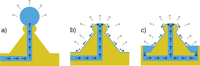
As described in the above section, microdroplets can be used as whispering-gallery mode resonators. However, it is very difficult to maintain these droplets at a stable size and shape. Part a) of the above figure shows how a micrdroplet may pin on the corner boundaries of the head of one our devices. Because the contact angle is too great and wetting is too low, the droplet is spheroid-shaped and the liquid cannot overcome the corner boundary. However, such a droplet is subject to extreme amounts of evaporation due to its large surface area to volume ratio. Additional liquid must be supplied at a very precise rate to counteract the effects of this evaporation. This precision is extremely difficult to maintain since the evaporation rate is dependent on many variables, many of which can be difficult to maintain.

We present an alternative technique for creating fluidic microresonators, which we call "water fountain resonators." Part b) of the figure shows a diagram of these resonators after being treated to be more wetting. Evaporation will still cause the film of liquid to fluctuate so active replenishing would be required. Part c) of the figure shows our passively replenishing fluidic resonator device. A 3D printed structure serves as the base for these resonators. The structure is then supplied with a liquid which will flow over the entire structure due to capillary action and high wetting. After flowing over the structure, the liquid is connected back to its supply reservoir. This results in a stable, thin film of recirculating liquid covering the structure. Like the microdroplet, this film is subject to evaporation, but because the water is constantly recirculating, the thickness of the film remains constant as long as there is liquid in the reservoir.

Part a) of the above figure shows a CAD model of the water fountain resonator. The device is roughly pawn shaped with a channel cut in the base and a vertical capillary in the center to allow liquid recirculation. The device is designed to be as smooth as possible, however it is known that the 3D printing process will not be able to prefectly recreate this smoothness. Part b) of the figure shows an SEM image of the device. This image clearly shows roughness and imperfections caused by the printing process. The roughness inherent in 3D printing has made it unsuitable for optical devices, but we overcome this issue by coating the device in liquid. Part c) shows the device coated in water. As can be seen, the film overcomes the rougness caused by the 3D printing process, resulting in a surface with optical quality.

Analysis Techniques

Upon successfully creating a structure with a reciculating film, analysis of the film is necessary. The above figure outlines the process. Using a microscope, we observe a dry device, and place the end of a bare optical fiber within the frame of view. The fiber has a known width of 125 microns, and by placing it in frame with the device, we are able to determine the exact scale of the pixels in the image. Removing the fiber, we take an image of the dry device then wet it and take still frames or video of the liquid film on the device. Three frames of interest are analyzed: a frame in which the fiber is visible, a frame of the dry device, and a frame of the device once liquid recirculation has been acheived. These frames are then converted to grayscale, and again converted to a binary image (details of the thresholding process are expained in the next section). The width of the fiber from the first frame is measured in pixels, and a conversion factor between pixels and microns is determined. Then the difference in size between the dry device and the wet device can be calculated.

By using and repeating this method, many useful metrics can be determined. We can determine where on the device the film is thickest or thinnest. Alternatively, by taking a long video, we can see how the film thickness is stable over time due to passive replenishing. These results are more fully explained in following sections.

Edge Uncertainty

We have developed our imaging techniques to be as accurate as possible; however, some uncertainty remains. The above image demonstrates how we account for the uncertainty in our measurements.

As described in the above section, in order to measure the film thickness, the video frames are converted to binary images. When converting a grayscale image to a binary image, a threshold value is selected. In a grayscale image, each pixel has a value ranging from 0 to 255, where 0 is black and 255 is white. When converting, any pixels with a value below the threshold value will be converted to white, while those above will be converted to black. Determining an appropriate threshold value is very important to making an accurate measurement. Since our measurements come down to a few pixels, slight variations in the threshold value can skew the results. To determine the ideal threshold value we select a box of pixels just inside and outside the edge feature for both dry and wet devices. We find the average value of the pixels inside each of the boxes and use the midpoint of the two values as the threshold value. This way, even if the lighting changes from image to image, the threshold value will be accordingly adjusted.

The uncertainty inherent in the process results from the way the image changes from light to dark gradually. These regions of pixel uncertainty are shown in the left portion of the above image for both the dry and wet device images. The lower left bars show the sample slices taken from the two inset images on the right. We used the average background grayscale value and the average device grayscale value to calculate an 80% region, which is marked in cyan above. The accepted edge of the device and device film is denoted in red and we determined this value using the thresholding method shown above. We accept uncertainty in the transition region shown, but due to consistency in our imaging process and the auto-thresholding method, the center of the transition region will always be selected, providing an accurate film thickness measurement between the two images.

Film Stability

As we have noted, our resonator devices require fluid film stability in order to be useful and refrain from transitioning through the mode spectrum. In the figure above we report film stability over the course of several hours. We took video and measurements as described above, and we intentionally disturbed the film by dropping water near the devices, supplementing the reservoir before allowing it to fully evaporate. The discrete pixel values will be explained below, but we note the standard deviation of this data set to be submicron. The mean value of the film thickness is 0.3 microns.

Stable Film in Depth

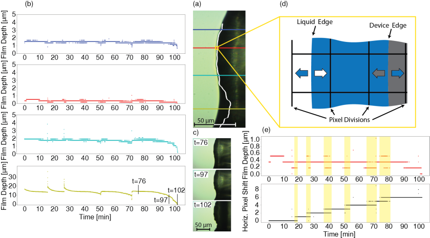
The red data set showing film stability is repeated on the left side of the figure above, along with three other measurement locations. Part a) shows a sample frame of the wetted device with four colored lines defining where the data sets in part b) were taken. We also superimposed the dry device onto the wet to show how the film is thickest at the neck (yellow data set) and thicker at certain pockets of water (blue and cyan data sets). We claim film stability at the red, blue, and cyan regions along the head of the device. The neck is much more susceptible to changes in film thickness as can be seen in the spikes when water was added. Near the end of the yellow data set are three time stamps which correlate to the three frames in part c) which show the evaporation process and how the reservoir itself must evaporate in order for the device film to evaporate.

Our devices are 3D printed using the digital light processing method. The resulting polymer has microscale voids that slowly fill with fluid as the water coating is adsorbed. Part d) is a diagram that shows how when the dry and liquid edges of the device are halfway between the camera pixel divisions the camera must choose which pixel to assign. This discretization error is enhanced because the resonator devices are constantly adsorbing water and expanding. Horizontal shift is shown in part e) where the device shifts 6 pixels throughout the 2 hour experiment. We used a mean squared error analysis to track the motion of our expanding device. Because of the pixel divisions of the camera shown in part d) the horizontal shift has regions of vascillation which are marked in yellow bars. The same red data set previously defined is aligned above the horizontal shift data with mirrored yellow bars to show that the pixels above and below 0.3 microns are an artifact of discretization and the film is actually quite stable.

Vertical Strain Fit to Fickian Curve

As stated above we tracked the motion of the device as water was adsorbed, both horizontal and vertical shift were apparent. The above figure shows how the vertical shift was much more drastic due to the bulk of polymer the device rests on. The red line is fickian curve for vertical straing due to adsorption which matches very well with the blue data that shows our measured vertical shift. The water disturbances are also apparent in this data, matching with the previous figures.

Now that we have characterized our devices and the remarkable curved, thin films we have created, we are much more prepared to implement them as optical resonators, which is our current research focus.

Liquid Microdroplet Resonators

Our previous work showed that we could maintain a stable film over a 3D printed surface, but no optical experiments were performed. Due to the innate smoothness of liquid films, we suspect a resonator based on our devices will exhibit a high quality factor (Q). We pursued this expectation and found we could create resonators with Q = 1.7 × 10⁶. The results were published in our paper—3D Printed Mounts for Microdroplet Resonators.

Figure 1

Our previous work demonstrated stable films over 3D printed bases; however, simulation shows that the optical mode penetrates the lossy 3D-printed resin, as shown in Fig. (1c), reducing the optical quality Q. To increase our Q the liquid film needs to be thicker so that the optical mode only penetrates the liquid. Fig. (1d) shows our simulation of the mode profile for several film thicknesses and compares the amount of optical power propagating inside the 3D printed material and outside of the material. The simulation suggests a high Q resonator requires a minimum film thickness of 8-10 μm. Due to oxygen plasma treatment, these thin film devices only have a film thickness of 2 μm.

Figure 2

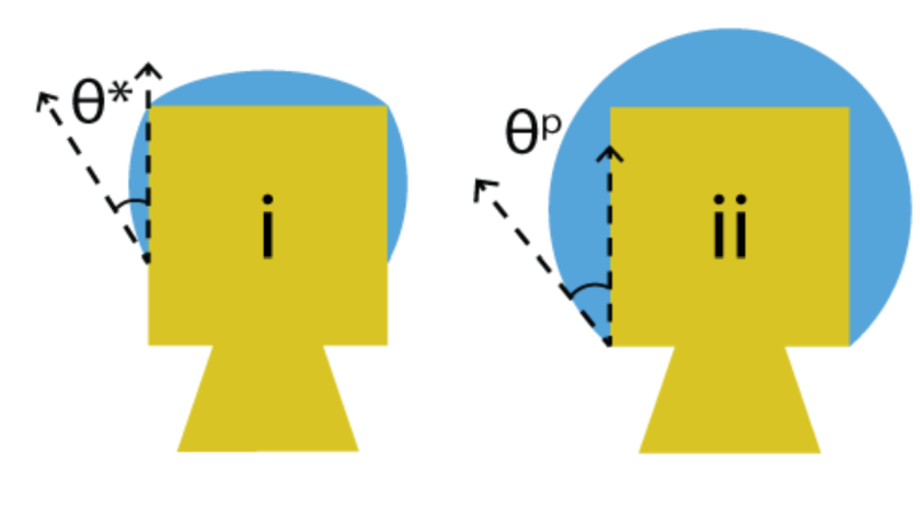
To increase the film thickness, we took advantage of corner pinning, meaning advancing a liquid cannot proceed around a corner boundary at the native contact angle, effectively being “pinned” at the corner. Devices exhibiting pinning used the rapid fabrication times and design flexibility of the 3D printing process. This enabled us to try various microfluidic systems, hydrophobic microstructuring, and unique geometries. We achieved the best results by leveraging corner pinning at the lower boundary of the device head by including a sharp undercut at the bottom of the device head. Fig. (2) shows that effect.

Figure 3

Fig. (3) shows an example device utilizing our final design. Fig. (3a) shows a profile view of the 3D printed mount, and Fig. (3b) shows a microdroplet supported by our 3D printed mount. The 3D printed mount also constrains the microdroplet size. Therefore scaling the 3D printed mount can constrain the droplet size to a specific range.

We create droplets on the device by dipping a bare optical fiber in liquid and then touching the fiber to the head of the device. Fig. (3c) shows the calculated fundamental mode for light polarized in the vertical direction (Z polarized) for a spherical paraffin oil droplet with a radius of 243.5 μm, this mode size is consistent with the modes in thin water film devices, however the droplets form a film that is approximately 50 μm thick.

Fig. (3d) shows the optical coupling setup of our experiments, which used a tapered optical fiber and a tunable laser. We taper the fiber using a heat-and-pull rig and monitor the optical throughput of the taper to pull the fiber until it becomes single mode. Then droplets are then carefully brought into close proximity to the fiber to couple into the resonant modes. Through careful cleaning and tensioning of the fiber, we maintained a stable coupling distance between the fiber and resonator, allowing us to control coupling efficiency, adjust polarization, and collect spectral data.

Figure 4

Using this stable coupling, we collected many data sets for varied resonator types using non-evaporating liquids. As the devices no longer utilize liquid recirculation, evaporation is present in the droplets. Future work will seek to adapt the mounts for use with water. Fig. (4a) shows a profile view of a droplet (radius of 257.9 μm) formed from a water/glycerol mixture. Fig. (4b) shows a resonant peak of the droplet, with a quality factor of Q = 1.7 × 10⁶, which suggests no penetration of the mode into the 3D printed material.

Figure 5

Most of our experiments were performed with paraffin oil. Fig. (5) shows resonant peaks of a paraffin oil microdroplet at both Z and R polarizations. Maxwell’s equations do not allow R polarized modes to have a continuous electric field across the edge of the droplet. As a result, the R polarized mode is more confined to the resonator than the Z polarized mode and has a smaller evanescent field, and thus a lower coupling efficiency, which we show in two Lorentzian-fitted plots in Fig. 5. Both polarizations showed peaks with Q in the range of 2 x 10⁵ to 5 x 10⁵.

Figure 6

In another experiment, we observed how the efficiency of the coupling changed when we adjusted the taper-droplet separation distance. Fig. (6) shows a single resonant peak of a paraffin oil droplet with data collected at many different coupling distances. We started by placing the droplet outside the coupling regime (d ≈ ∞). Then the droplet was carefully moved closer to the fiber until we observed resonant peaks. We acquired spectral data for each polarization (Z and R), a process that took just under a minute to complete. Then we moved the resonator closer to the fiber until the droplet came into contact with the fiber. At a distance of 690 nm from the fiber, the coupling is only about 2% efficient, while at 30 nm the efficiency is near 50%. Fig. (6) also has three other features. First, there is a slight red shift in the resonant wavelength as the coupling distance decreases, which the thermal dependence in the refractive index of the oil likely causes. Second, the resonant peaks split into doublets, which is due to coupling between modes with significant overlap. In smaller droplets fewer modes are supported, and we observed fewer doublet peaks. Finally, the data contains off-resonance features, which are strongly correlated with the coupling to higher-order modes in the droplet.

One of the benefits of using our 3D-printed mounts to support the droplets is the mounts’ versatility. In conjunction with our precision coupling method, this versatility allows for various microdroplet resonators to be tested with no changes to the tapered fiber or any of the other optical components, ensuring that all changes are caused by the droplet. The mounts can be used with various liquids, and the size and shape of the mounts can easily be changed. In our experiments, our mounts allowed us to create microdroplets of paraffin oil, silicone oil, and glycerol with diameters between 300μm and 600μm. Furthermore, we created mounts with racetrack-shaped cross sections, which supported ellipsoidal droplets of eccentricities as extreme as 0.58.

In conclusion, we present a unique 3D printed mount for optical microdroplet resonators. These mounts provide a robust and easy-to-use method for supporting microdroplet resonators while still allowing control over the droplet position, shape, and size. In our experiments, we found that the main deterrent to creating smaller droplets was the difficulty of placing the liquid on the mount by hand. We believe that with a more precise delivery method, the droplet size could be decreased dramatically. In our future work, we will also integrate 3D printed microfluidic systems that will allow us to deliver liquid to smaller devices and dynamically change the nature of the liquid used in the microdroplets by changing its volume or introducing analytes.